Please ask about problems and questions regarding this tutorial on answers.ros.org. Don't forget to include in your question the link to this page, the versions of your OS & ROS, and also add appropriate tags.

Incorporate dynamic obstacles

Introduction

This tutorial demonstrates how dynamic obstacles can be included in the teb_local_planner.

In a previous tutorial you learned how to provide user-supplied obstacles via an array of costmap_converter/ObstacleMsg messages. The message definition includes a geometry_msgs/TwistWithCovariance field called velocities which captures the current centroid's velocity. Currently, only linear.x and linear.y are processed by the teb_local_planner package.

Write a Simple Dynamic Obstacle Publisher

In the following, we will create a small python node that publishes a dynamic obstacle. For the planning part, we will run the test_optim_node described in the tutorial Set up and test Optimization. Alternatively, you could also test your publisher using a properly configured navigation launch file according to Configure and run Robot Navigation.

Create a python node called publish_dynamic_obstacles.py:

   1 #!/usr/bin/env python
   2 
   3 import rospy, math, tf
   4 from costmap_converter.msg import ObstacleArrayMsg, ObstacleMsg
   5 from geometry_msgs.msg import Point32, QuaternionStamped, Quaternion, TwistWithCovariance
   6 from tf.transformations import quaternion_from_euler
   7 
   8 
   9 def publish_obstacle_msg():
  10   pub = rospy.Publisher('/test_optim_node/obstacles', ObstacleArrayMsg, queue_size=1)
  11   rospy.init_node("test_obstacle_msg")
  12 
  13   y_0 = -3.0
  14   vel_x = 0.0
  15   vel_y = 0.3
  16   range_y = 6.0
  17 
  18   obstacle_msg = ObstacleArrayMsg() 
  19   obstacle_msg.header.stamp = rospy.Time.now()
  20   obstacle_msg.header.frame_id = "odom" # CHANGE HERE: odom/map
  21   
  22   # Add point obstacle
  23   obstacle_msg.obstacles.append(ObstacleMsg())
  24   obstacle_msg.obstacles[0].id = 99
  25   obstacle_msg.obstacles[0].polygon.points = [Point32()]
  26   obstacle_msg.obstacles[0].polygon.points[0].x = -1.5
  27   obstacle_msg.obstacles[0].polygon.points[0].y = 0
  28   obstacle_msg.obstacles[0].polygon.points[0].z = 0
  29 
  30   yaw = math.atan2(vel_y, vel_x)
  31   q = tf.transformations.quaternion_from_euler(0,0,yaw)
  32   obstacle_msg.obstacles[0].orientation = Quaternion(*q)
  33 
  34   obstacle_msg.obstacles[0].velocities.twist.linear.x = vel_x
  35   obstacle_msg.obstacles[0].velocities.twist.linear.y = vel_y
  36   obstacle_msg.obstacles[0].velocities.twist.linear.z = 0
  37   obstacle_msg.obstacles[0].velocities.twist.angular.x = 0
  38   obstacle_msg.obstacles[0].velocities.twist.angular.y = 0
  39   obstacle_msg.obstacles[0].velocities.twist.angular.z = 0
  40 
  41   r = rospy.Rate(10) # 10hz
  42   t = 0.0
  43   while not rospy.is_shutdown():
  44     
  45     # Vary y component of the point obstacle
  46     if (vel_y >= 0):
  47       obstacle_msg.obstacles[0].polygon.points[0].y = y_0 + (vel_y*t)%range_y
  48     else:
  49       obstacle_msg.obstacles[0].polygon.points[0].y = y_0 + (vel_y*t)%range_y - range_y
  50 
  51     t = t + 0.1
  52     
  53     pub.publish(obstacle_msg)
  54     
  55     r.sleep()
  56 
  57 
  58 if __name__ == '__main__': 
  59   try:
  60     publish_obstacle_msg()
  61   except rospy.ROSInterruptException:
  62     pass

Here we skip breaking the code down since creating a publisher and publishing messages is explained well in the beginner tutorials section (see here).

Now run the teb_local_planner test_optim_node in combination with rviz:

roslaunch teb_local_planner test_optim_node.launch

In the following, we assume that your package containing the python script is called mypublisher. Make sure that your script is marked as executable (chmod +x publish_dynamic_obstacles.py). Open a new terminal and run your newly created python script:

rosrun mypublisher publish_dynamic_obstacles.py

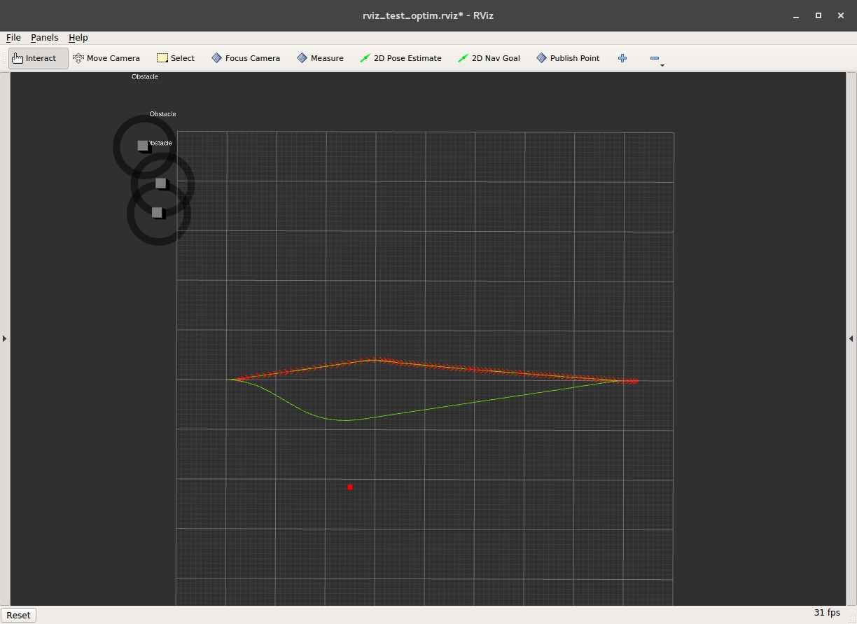
You should now see a visualization (rviz) that should look similar to the one in the previous tutorials, in particular, you should be able to see the default test_optim_node obstacles (interactive markers) and the new moving (dynamic) obstacle

However, the dynamic obstacle feature is not yet enabled in the teb_local_planner/test_optim_node. We will do this in the next section.

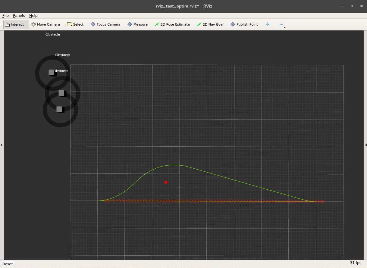
Before you proceed, please move the interactive markers far away from the planning scene, like in the following figure:

Set up the Planner for Considering Dynamic Obstacles

Start the rqt_reconfigure node in a new terminal:

rosrun rqt_reconfigure rqt_reconfigure

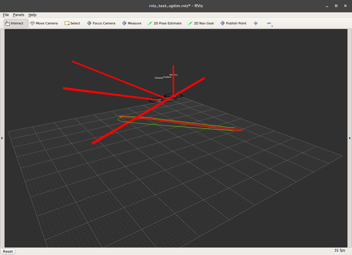
Now activate the check-box for parameter include_dynamic_obstacles (obstacles section). The teb_local_planner now utilizes a constant-velocity-model to predict the obstacles future motion. You should now recognize that the ego-trajectory avoids the obstacle based on the spatio-temporal distance rather than based on the current obstacle position (see the next figure). Note, it is important that the velocity estimation is accurate and that the constant-velocity assumption is fairly satisfied.

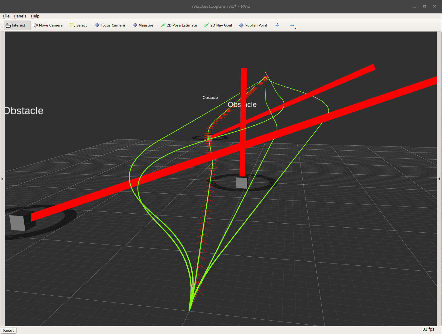
You can also visualize the temporal evolution of the planned and predicted velocities if you adjust parameter visualize_with_time_as_z_axis. You can set the parameter value now to 0.1. The z-axis in rviz is now interpreted as time-axis scaled by the specified factor. Here you can also see how the homotopy-class-planning (planning in distinctive topologies) takes the dynamic obstacle predictions into account:

You might have noticed, that two of the interactive marker obstacles of the test_optim_node are defined with a non-zero velocity. Feel free to move them into the planning scene and observe how the planner performs:

Note, the teb_local_planner defines some dedicated optimization weights for dynamic obstacles. Refer to the list in the next section.

Related Parameters

Parameters that influence planning with custom obstacles are listed here (refer to the Node API for more details):

• ~<name>/min_obstacle_dist: Desired minimal distance from (static and dynamic) obstacles

• ~<name>/inflation_dist: Non-zero cost region around (static) obstacles

• ~<name>/include_dynamic_obstacles: Specify whether the motion of dynamic obstacles should be included (constant-velocity-model) or not.

• ~<name>/dynamic_obstacle_inflation_dist: Non-zero cost region around (dynamic) obstacles

• ~<name>/include_costmap_obstacles: Deactivate costmap obstacles completely

• ~<name>/costmap_obstacles_behind_robot_dist: Maximum distance behind the robot searched for occupied costmap cells.

• ~<name>/obstacle_poses_affected: Specify how many trajectory configurations/poses should be taken into account next to the closest one.

• ~<name>/weight_obstacle: Optimization weight for keeping a distance to static obstacles.

• ~<name>/weight_inflation: Optimization weight for inflation costs of static obstacles.

• ~<name>/weight_dynamic_obstacle: Optimization weight for keeping a distance to dynamic obstacles.

• ~<name>/weight_dynamic_obstacle_inflation: Optimization weight for inflation costs of dynamic obstacles.

• ~<name>/footprint_model: The robot footprint model